
As an expert in this sector, I’m thrilled to share my inner secrets for understanding Microsoft Excel software in this thorough guide. Whether you’re new to Excel or trying to improve your skills, I’ll show you how to get the most out of this advanced spreadsheet tool.
You will progress from fundamental functionalities to complex data analytics and visualizations. Prepare to modify and streamline your operations like never before and become a true Excel power user. Let us get right to it!
What is Microsoft Excel?
Microsoft Excel is widely used in the business world as a powerful spreadsheet software program. It is utilized for data entry and management, creating charts and graphs, as well as handling project management tasks. This tool allows you to effortlessly format, organize, visualize, and calculate data.
How to Download Microsoft Excel
Downloading Microsoft Excel is incredibly easy. Start by making sure that your PC or Mac meets Microsoft’s system requirements. After you’ve confirmed, go ahead and log in to start the installation process for Microsoft 365.
After signing in, just follow the customized steps for your account and computer setup to effortlessly download and launch the program.
Let’s say you’re navigating through a Mac desktop environment. Navigate to Launchpad or explore your application folder. Locate the Excel icon and give it a click to effortlessly open the application.
Key Takeaway
- Excel is a versatile and powerful spreadsheet program used widely in business for data analysis, visualization, and more. It has many capabilities to help organize, calculate, and present data.
- Core skills like entering data, formulas, sorting, filtering, freezing panes, and using functions like SUM and AVERAGE are fundamental building blocks in Excel. Master these early on.
- PivotTables, charts, macros, and tools like VLOOKUP allow more advanced analytics and automation. Dedicate time to learning these areas.
- Formatting cells, conditional formatting, and other stylistic tools help create more polished, professional spreadsheets. Don’t neglect the design.
- Learn shortcuts, fill handles, and features like Format Painter to work faster and boost productivity in Excel. Streamline repetitive tasks.
- Excel helps sales, marketing, finance and other roles slice and dice data to drive insights and strategy. Become a power user to stand out.
- Include Excel proficiency prominently in resumes and cover letters. Quantify experience in years and highlight formal training.
- Excel skills translate to workplace results. Invest time to truly master this versatile program for a career edge.
Who Uses Microsoft Excel?
Throughout my various professional experiences in the finance industry, I have found Excel to be an essential tool that I cannot do without. Consider the realm of investment banking, where Excel reigns supreme for constructing complex financial models and analyzing financial data.
Accountants also utilize Excel’s capabilities to carefully track and document financial details while creating budgets and producing detailed reports. In addition to the finance sector, data analysts from various industries often depend on Excel for its powerful features in data analysis and visualization.

Microsoft Excel Spreadsheet Basics
At times, Excel appears almost too good to be true. Looking to merge information from various cells? Excel is more than capable of handling it. Want to effortlessly apply formatting to multiple cells at once? Indeed, Excel is also capable of performing that task.
Allow me to commence this Excel guide by covering the fundamentals. Once you have a solid grasp of these functions, you’ll be well-prepared to navigate your way through.
Blank Excel Workbook
As soon as the application is opened, a new workbook can be created. When you open a workbook, you’ll notice that a blank worksheet is displayed and it looks like this:
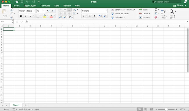
Starting with a blank workbook, one can effortlessly tackle essential Excel tasks.
Data Entry
Inputting data into Excel is a breeze. Select the cell where you wish to input the information and begin typing.
Inserting Rows or Columns
As one works with data, there may come a point where the need arises to include additional rows and columns. Doing this one by one would be incredibly monotonous. Fortunately, there is a more convenient method.
If you want to add multiple rows or columns to a spreadsheet, simply highlight the desired number of pre-existing rows or columns. Next, right-click and choose the option “Insert.”
In this example, I added three rows to the top of my spreadsheet.
Freeze Rows or Columns
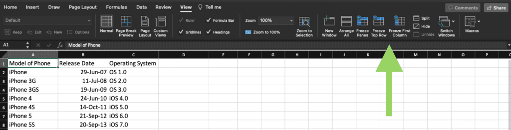
Freezing rows and columns has completely transformed my experience when reviewing large datasets or tables. When I want to keep headers visible as I scroll down, I just open the “View” menu and click on “Freeze Top Row”. It’s a simple and effective way to ensure that the headers stay in place. I am able to consistently observe the context of the data I am analyzing.
The “Freeze First Column” option is incredibly useful for ensuring that ID numbers or categories remain fixed in place as I navigate horizontally to analyze trends across different fields. Thanks to Excel’s freeze panes feature, I can easily keep track of field names and references without the need to constantly switch back and forth.
Using it saves me a ton of time and prevents any mistakes! I highly recommend that all analysts utilize these freeze-pane views in Excel. They will greatly enhance the efficiency and ease of your data review and analysis.
Hide Columns and Rows
Before sharing reports with stakeholders, I frequently find it necessary to hide specific columns or rows. For instance, there may be a need to hide confidential cost data or preliminary calculations. It’s simple to hide columns.
All I have to do is select the columns, right-click the header, and then simply choose the “Hide” option. You can hide the rows in the same manner.
I am able to maintain a comprehensive working spreadsheet while presenting only the crucial final numbers and figures to others. I can effortlessly toggle hidden columns and rows on and off with just a few clicks as I work. It’s a simple trick that keeps my spreadsheets clean for presentation without losing any background details.
Autofill
The autofill feature in Excel greatly enhances my productivity. When it comes to swiftly duplicating values, formulas, or series across cells, the fill handle is my trusty tool of choice. When I want to extend a series of consecutive numbers or dates, I just click the cell with the first value, then use the fill handle (the little blue square in the bottom right corner) to drag across the desired range. Excel automatically continues the pattern.
Autofill effortlessly applies the references correctly across new rows or columns, eliminating the need for tedious copying and pasting. It’s like having a personal assistant that takes care of all the formulaic details.
By simply dragging the fill handle, I effortlessly populate a vast spreadsheet area with perfect evenness in a matter of seconds. Autofill is incredibly efficient and ensures accurate data entry without any manual effort.
First, select which cells you wish to be the source. Next, look for the fill handle in the cell’s lower right corner. Then, either drag the fill handle over the cells you wish to fill or simply double-click.
Filters
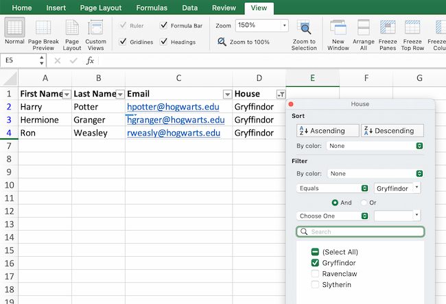
Filtering is one of my go-to Excel abilities for processing enormous datasets and identifying significant insights. Rather than sifting through hundreds of useless rows, I can rapidly narrow the view to only the most important records. The filter arrows adjacent to column headers are really useful; with a few clicks, I can organize and display/hide data points based on criteria such as dates, geographies, and metrics.
Before distributing filtered reports to stakeholders, I make sure to copy the visible cells to a new sheet and delete the underlying hidden rows. This filtering procedure significantly improves the efficiency of my analysis. I can accurately identify trends, outliers, and patterns.
Learning how to filter properly in Excel is essential for any analyst or power user dealing with large datasets. It streamlines your process and elevates your data-interrogation abilities!
Let’s take a look at the example below.
Sort
Excel’s sort feature helps me organize my campaign contact lists, customer data, and other records exported from other platforms. With ever-growing databases, a fast A-Z or Z-A sort keeps everything properly alphabetized and easy to find. Simply pressing the Sort button in the Data tab quickly arranges any list or table precisely.
I especially love the ability to switch between ascending and descending sorting based on my requirements. No more searching endlessly through messy spreadsheets! Sorting campaign data correctly in Excel is a key efficiency hack for any marketer who manages many outreach lists.
Taking a minute to sort saves me a lot of time browsing and searching for the right contacts or information when planning campaigns or running reports. It’s a simple yet transformative organizational tool.
Remove Duplicates
When it comes to creating master CRM and contact lists, duplicate records are my worst nightmare. They skewed all aggregated stats and information. Fortunately, Excel’s Remove Duplicates feature is an absolute game changer for consolidating clean data sets.
Whether it’s duplicate email addresses in a lead list or duplicated company names across regions, I can simply highlight the column and select Remove Duplicates from the Data menu. In a single click, this mercilessly reduces any table to its unique values or rows. There will be no more manual scanning for repetitions across lengthy spreadsheets!
With clean, duplicate-free CRM data, my analysis and reporting are infinitely more accurate. My productivity increases without wasting time repairing messy, duplicated data. Every sales operations professional should know this approach for compiling immaculate contact lists and efficiently removing unnecessary records when integrating several data sources.
Remove Blank Rows or Columns
To remove blank rows, you can simply navigate to the “Find & Select” option located on the Home tab. Select the “Go To Special” option from the drop-down menu to access a pop-up window with various choices. Here, you have the option to click on “blanks” in order to select all the empty cells. Next, navigate to the Delete menu and select the option “Delete Cells.”
The remaining cells can be shifted in any direction: up, down, left, or right. After deleting rows in the middle of our data set, it is necessary for the remaining rows to shift up.
Sum
Excel formulas are essential for me to analyze product sales and performance trends. Although AutoSum is convenient for basic calculations, I prefer utilizing more advanced formulas like SUMIFS to dynamically aggregate data.
To calculate the total monthly sales for each product, I would simply click on a blank cell and input “=SUMIFS” along with the range of sales data, followed by the criteria for the month and product. It’s all about getting the formulas structured just right so that the values are summed only when every single criterion is satisfied. I have a deep understanding of the formulas needed to generate custom reports on category trends, customer cohorts, rolling averages, and more.
The possibilities are truly limitless! Mastering the art of constructing formulas has elevated my data analysis skills to new heights. I have the ability to effortlessly work with and analyze extensive datasets, allowing me to uncover valuable business insights with ease.
For this example, we want to find the total number of each product sold in January, February, and March. So, we’ll use the formula:
When we click enter, we’ll see the total sales across those three months.
Here’s a helpful tip: When you move your cursor over the bottom right corner of the cell containing the formula, you’ll notice a plus sign. Simply click and drag down to effortlessly apply the same function to every row and let it automatically fill in.
Paste Special
Converting the items in a row of data into a column (or vice versa) can be quite beneficial. Copying and pasting each individual header would be quite time-consuming.
Furthermore, one must be cautious of inadvertently succumbing to the common and regrettable pitfall of human error when working with Excel.
Why bother making any of these mistakes when you can let Excel handle it for you? Here’s an example for you to consider:
If you want to use this function, simply highlight the column or row you wish to transpose. Next, simply right-click and choose the option “Copy.”
Afterwards, choose the cells where you’d like the initial row or column to start. Simply right-click on the cell and choose “Paste Special.”
Once the module pops up, simply select the option to transpose.
Paste Special is an incredibly handy function. Within the module, you have the option to select between copying formulas, values, formats, or even column widths. It’s particularly useful when it comes to transferring the outcomes of your pivot table into a chart.
Text to Columns
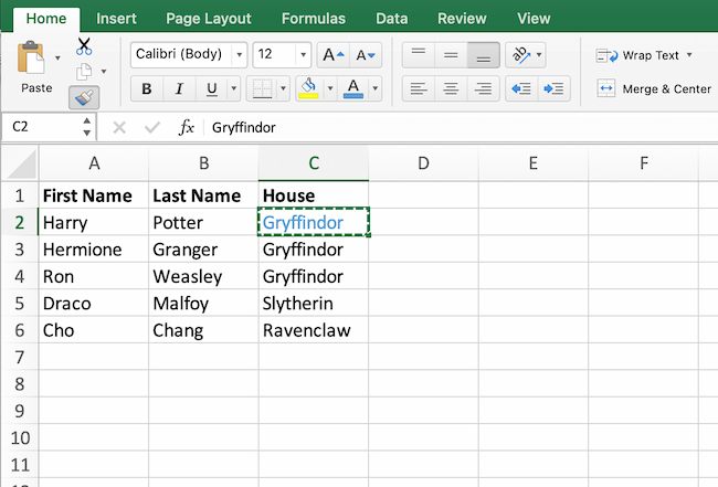
How can one separate information from a single cell into two separate cells? For instance, perhaps you wish to extract the name of a company from an email address. Perhaps you’re looking to split a person’s complete name into a first and last name for your email marketing templates.
Thanks to Microsoft Excel, both options are now within reach. To begin, select the column that you wish to divide. After that, navigate to the Data tab and choose the option “Text to Columns.” You’ll see a module pop up with additional details. To begin, you have the option to choose between “Delimited” or “Fixed Width.”
- Delimited means you want to break up the column based on characters such as commas, spaces, or tabs.
- Fixed Width means you want to select the exact location in all the columns where you want the split to occur.
Choose “Delimited” to split the full name into the first name and last name.
Now, it’s time to select the delimiters. There are various options for delimiters, such as tabs, semicolons, commas, spaces, or other characters. (As an illustration, “something else” might refer to the “@” symbol commonly used in email addresses.) Let’s select the setting for this example. Once you’ve made your selections, Excel will provide you with a preview of how your new columns will appear.
Once you’re satisfied with the preview, simply click on “Next.” You have the option to select Advanced Formats on this page. Once you’ve completed the task, simply click on the “Finish” button.
Format Painter
Adjusting the fonts, colors, and borders of each cell can be quite time-consuming. The Format Painter is incredibly useful and has become an indispensable tool for me! With just a few clicks, it’s incredibly easy to replicate formatting from one cell to entire rows or columns.
Simply choose the source cell, click on the paintbrush icon, and effortlessly glide over the target cells to seamlessly match their style. I frequently rely on Format Painter to ensure consistency in my headings, emphasize totals, and apply table borders; there’s no limit to its usefulness. Styling cells is no longer a tedious task! Formatting might appear insignificant, but well-crafted, professional spreadsheets leave a lasting impact.
Average
The average function functions similarly to the sum function, but instead, we utilize the following formula:
=AVERAGE(B2,C2,D2)
Concatenate
Concatenate enables the seamless stringing together of cells. This function allows you to effortlessly combine customer names when their first and last names are in separate cells, or merge cities and states that are organized in different columns. Here’s a simple formula for concatenating:
=CONCATENATE(
You can then add specific cell coordinates in whichever order you need them. To include spaces between details, simply add a comma and a space between the cells. You can also include any other elements within quotation marks, like commas or phrases.
In this example, we want to make a sentence saying where a music artist was born. So, we’ll use this formula (# stands for the desired row number):
=CONCATENATE(B#,” “,A#,” was born in “,C#,”,”,D#)
Logic Functions
Logic functions adhere to rational thought processes. Take the case of a car that happens to be red. In this scenario, it can be described as a red car. These functions can be quite handy when it comes to swiftly organizing data and forming assessments.
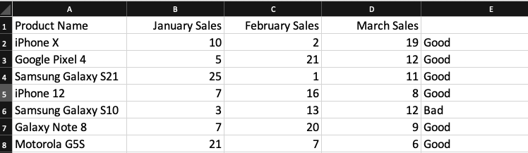
The IF function has the ability to provide a precise response or value when a cell satisfies a particular condition. Let’s take a look at which Q1 products had sales exceeding 30 units. Well, the formula we used was:
=IF(SUM(B#,C#,D#)>30, “Good”, “Bad”)
This formula basically states that if the total sales for January, February, and March exceed 30, the cell will display “Good”. If not, write “Bad.”
Based on the formula, the results obtained are as follows:
The AND logic function operates in a comparable manner. Simply input the desired conditions for the cells, and the system will promptly provide a response of either TRUE or FALSE. For instance, when you input the given data, =AND(B2>5,C2<5), the result will be TRUE. This is because B2 is greater than five and C2 is less than five.
Vlookup
With the VLOOKUP function, you can effortlessly locate precise information within a dataset.
To use this function effectively, you’ll need to provide specific details. Specify the desired outcome, the location to search, the column number with the relevant data, and whether you prefer an approximate or exact match. For approximate matches, you can input either 1 or TRUE. On the other hand, exact matches require 0 or FALSE.

In this example, I was searching for the employee with ID number 3856 in the table that extends from cell A2 to cell F8. We requested the last name to be extracted from column No. 2, with the requirement of an exact match.
Pivot Tables
Organizing and analyzing large data sets within Excel becomes a breeze with the help of a pivot table. To create a pivot table, simply navigate to the Insert tab in the navigation bar and click on “Insert Pivot Table.”
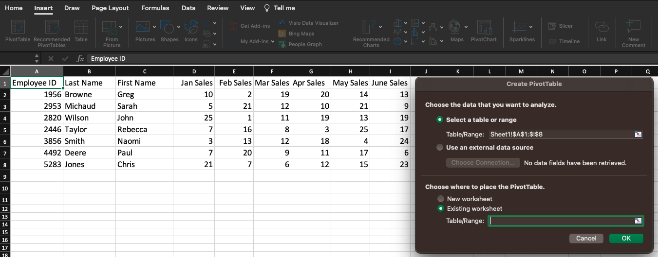
You have the option to choose the specific range of data you want to include in the pivot table. Additionally, you can decide whether you want to create the table on the same worksheet or in a new sheet. After choosing your data and the table destination, a sidebar will appear:
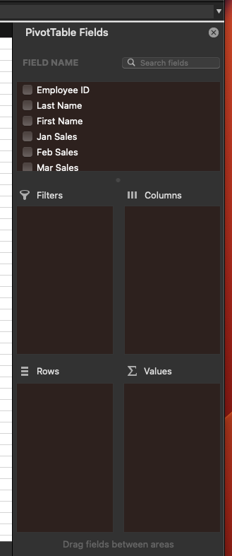
With this sidebar, you have the freedom to select the columns of data you prefer and determine their placement within the pivot table. For instance, if you prefer arranging employee first names as rows and sales numbers as columns, you can easily select those fields and effortlessly drag them to the corresponding areas in the sidebar.
After arranging the data to your liking, you have the freedom to alter its presentation. As an illustration, this pivot table showcases employee ID numbers as the row labels, while the columns represent the sales for January, February, and March. The table automatically displays the total for each column (or the total for each month’s sales).
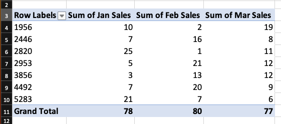
It is possible to alter the way in which the data is summarized. In order to view the average sales for each month, we simply need to right-click on the desired data in the sidebar, proceed to select “Field Settings,” and then choose “Average” from the “Summarize by” menu.
Excel Formulas
By now, I’m sure you’re quite familiar with Excel’s interface and effortlessly navigate through your spreadsheets with lightning-fast commands.
Now, let’s delve into the fundamental use case for the software: Excel formulas. With Excel, you have the power to effortlessly perform basic arithmetic operations such as addition, subtraction, multiplication, and division on any set of data.
- To add, use the + sign.
- To subtract, use the – sign.
- To multiply, use the * sign.
- To divide, use the / sign.
- To use exponents, use the ^ sign.
Remember, all formulas in Excel must begin with an equal sign (=). Use parentheses to make sure certain calculations happen first. For example, consider how =10+10*10 is different from =(10+10)*10.
Besides manually typing in simple calculations, you can also refer to Excel’s built-in formulas. Some of the most common include:
- Average: =AVERAGE(cell range)
- Sum: =SUM(cell range)
- Count: =COUNT(cell range)
Also note that series’ of specific cells are separated by a comma (,), while cell ranges are notated with a colon (:). For example, you could use any of these formulas:
- =SUM(4,4)
- =SUM(A4,B4)
- =SUM(A4:B4)
How to Show Excel Skills on Resumes
Including Excel in your skills section on your resume is a great idea. Nevertheless, there are several approaches to accomplishing this:
- List specific abilities you have that rely on using Excel, such as making financial models.
- Explain how many years of experience you have with the program.
- Describe specific Excel functions you have experience with, such as data visualization, pivot tables, and VLOOKUP functions.
- Show your years of experience with the Microsoft Office 365 suite.
Moreover, please indicate whether you have completed a formal Excel course. In your cover letter, it can be effective to mention specific, relevant experiences, such as your proficiency in Excel and other software. Mastering Excel is a valuable skill that should be confidently highlighted in relevant contexts.
Here is a free template to help you create a mind-blowing resume:
Conclusion
Excel is a valuable resource for any small business. Whether you work in marketing, human resources, sales, or service, these Microsoft Excel tips can help you perform better.
Excel can help you enhance your efficiency and production. You can identify new trends and organize your data to gain useful insights. It can help you understand your data and complete your daily chores more efficiently.
It only requires a little know-how and some time with the software. So start learning and prepare to improve.
- Project Management Tools Excel Free: All You Need To Know, Types, and Free Tools To Use
- FREE PROJECT MANAGEMENT TOOLS EXCEL: All You Need to Know
- 15 BEST ACCOUNTING SOFTWARE TO USE IN 2023
- Cash Flow Forecasting: Meaning, Methods, Tools, Models (+ Detailed Templates)
- Who Benefits Most From a Master’s Degree?